How to Compare Lists of Data and Find Differences in Excel

Generally Conditional Formatting allows you to format cells that meet a given condition or criteria. But it can be used to highlight values in a list that do not appear in another, too:

To do this:

1. Select the cells that you wish to apply Conditional Formatting to
2. From the Home tab click on the Conditional Formatting Button
3. Choose New Rule
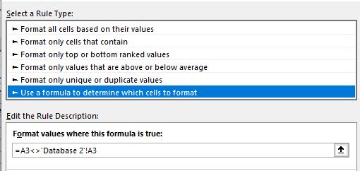
   The New Formatting Rule (dialog box appears)
4. Select use a formula to determine which cells to format
5. Enter the formula =A3<>'Database 2'!A3
6. Change the formatting of the cells (as required
7. Click OK.

If your sheets are in the same workbook you will need to show both sheets on the screen at the same time.

To show both sheets in same workbook:

1. Click View Tab > New Window (opens same sheet a second time)
2. Go back to View Tab > Arrange All > Select Vertical > Click OK

You can also have a scenario where the sheets are in different workbooks but you can’t use Conditional Formatting across workbooks. It will need a logical formula to find the differences.

Find out more on our Excel Level 4 course

Join us on our interactive and engaging Expert Excel Core Level 4 full-day course (split over two half-days) to learn how to build more complex calculations that will deepen your understanding and help you feel more confident with problem-solving in Excel.

Related blogs

• How to Use Conditional Formatting in Microsoft Excel — Get started with Conditional Formatting in this two-minute video.
• How to Colour Code Your Data Validation Dropdown List in Excel — Adding colour to certain elements within a spreadsheet can create visual appeal and increase user accuracy when it comes down to interpreting your data. Find out how in this blog.
• How to Use the Excel Dynamic Array FILTER Function — What do you do if you want to look up multiple criteria that returns all match results, not just the first match? Then the new Excel Dynamic Array FILTER formula will come to the rescue!