How to Use the Data Consolidation Feature in Excel

Data Consolidation allows you to gather together your data from separate worksheets into a master worksheet. In other words, the Data Consolidation function takes data from a series of worksheets or workbooks and summaries it into a single worksheet that you can update easily.

The trouble is, working with Data Consolidation can be tricky! Don’t be put off. Data Consolidation is an incredibly useful tool that help you understand and present your data quickly and easily. The screen may look daunting but like all great things, good planning is the key.

This example contains some tips from Edmund, one of our Excel experts, and will help you decide how to organise your data before you start summarising it to get easily understandable results.

Here we look at:

1. Consolidating data from multiple worksheets to one summary within the same workbook.
2. Consolidating data from multiple workbooks to one summary in a new workbook.

NOTE: The following processes will work in Excel versions: 2007, 2010, 2013 and 2016. If you are using an older version (Excel 2003 or older), this tip may not work for you.

Consolidate data in multiple worksheets within the same workbook

In our example, we have data for 3 years expenditure on tea, coffee and milk. The data is broken down into quarters and stored in one year per worksheet in one workbook. We can create a ‘Consolidated Summary’ sheet which will show expenditure by year and quarter. It does not matter if the data has the same arrangement of columns and rows or not. Excel will sort that out for you. Amazing!

Year 1 worksheet

Year 2 worksheet

Year 3 worksheet

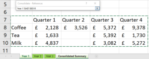
As you can see, Years 1, 2 and 3 each have different arrangements of columns and rows. There is no tea in Year 2; in Year 3 the first quarter appears at the end of the table, there is no Quarter 2 and the Quarters are not in order. The ranges you consolidate do not have to be of the same size in each worksheet, the number of rows or columns might be different from sheet to sheet. And yet, you can still consolidate the data into a summary sheet. How incredible is that!

Consolidation steps:

To start using the Data Consolidation tool, you need to select an empty sheet in the workbook as your master worksheet or add a new one if necessary. The worksheet is renamed ‘Consolidated Summary’.

Select the upper-left cell of the area where you want the consolidated data to appear.

On the Ribbon, Choose Data > Consolidate to view the Consolidate dialog:

In the Function box, click the summary function that you want Excel to use to consolidate the data. As you will see from the drop-down, there are 11 functions to choose from. For our data we want to add up the values so we’ll set the Function to Sum. 

Click in the Reference area and select the first data range to consolidate – to do this you will need to click the Sheet tab i.e. “Year 1” and then drag over the data (including row and column headings) and then click the Add button to add this first set of data to the consolidation dialog.

Continue in the same way by clicking on the next sheet, highlighting the data, and clicking on the Add button until all your data and worksheets appear in the References section of the dialog e.g. “Year 2” and “Year 3”. 

Top Tip: You can name your ranges before you start the Consolidation process. If you name each range then, when you create the consolidation, place your cursor in the Reference field, press F3 and then choose the range from the list in the Paste Name dialog.

To indicate where the labels are located in the source ranges, select the check boxes under Use labels in: either the Top row, the Left column, or both. In this example, Top row is the name of the quarters, i.e. Quarter 1, Quarter 2, etc. and the Left Column are the list of items, i.e. Coffee, Tea and Milk.

Automatic vs. Manual updates: If you want Excel to update your consolidation table automatically when the source data changes, select the Create links to source data check box. If unchecked, you can still update the consolidation manually.

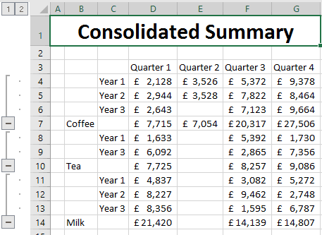
When you click OK, Excel summarises all the data into your new sheet as your master worksheet (Consolidated Summary).

You’ll immediately notice a change to the Excel worksheet that you may never have seen before. You will see grouping tools down the left of the screen which you can use to display and hide the data. Next to rows 7, 10 and 14, there are plus signs. This signifies that cells are part of a group that is currently collapsed. Clicking on the plus sign will expand the group and there is a line connecting these rows to the left:

You’ll find that the second column (Column C) of data shows the name of the workbook (Core Excel Level 2) that contains the data. You can hide this column if you want to, by right clicking it and choosing Hide. This simply hides the column so the data is there should you need to refer to it later on.

Copying your worksheets to a new workbook

Here’s another time when pre-planning will be your friend.

When you look at your Consolidated Summary, you will see that there are some entries which are not helpful. For instance, range C4:C6 shows only the name of the workbook, so we cannot immediately see where the figures in the range D4:G6 come from.

If you wish to show the location of the source data on the summary sheet, I strongly advise you to separate all worksheets to individual workbooks before you apply the data consolidation. Let’s look at how to do this.

We’re going to copy the selected worksheet into a new workbook, so select (new book) from the To book drop-down list. Select the Create a copy check box. Because we’re creating a new workbook, there are no worksheets in the Before sheet list before which we can insert the copied worksheet. It will be the only worksheet in the new workbook.

Click OK. A new workbook is created and the worksheet is copied into it. If you chose to move the worksheet, it will no longer be in the original workbook. Save the current workbook by the name of the worksheet that you copied to i.e. “Year 1.xls”.

Continue creating new workbooks for each year e.g. “Year 2” and “Year 3” to “Year 2.xls” and “Year 3.xls” respectively. Yes, this is tedious, especially if you have a lot of worksheets, but you’ll thank me in the end!

Consolidate data from multiple workbooks to one new workbook

Make sure all the individual workbooks you wish to consolidate are currently open.

Open a new, blank workbook as your master worksheet or add a new one if necessary. The worksheet is renamed as “Consolidate Summary” and save this workbook with a name e.g. Summary.xls.

Select the upper-left cell of the area where you want the consolidated data to appear.

On the Ribbon, Choose Data > Consolidate to view the Consolidate dialog

We now simply proceed as we did in the first example, the only difference being we are selecting data ranges from different workbooks instead of different worksheets.

When you click OK, Excel summarises all the data into your new master worksheet (Consolidated Summary).

Here you will see the same data as in the first example, except displayed in a much more helpful way – Column C now shows the name of the workbook that contains the data.

Related Blogs

• Save Time in Excel with Autofill - Learn how to use the useful tool Autofill. Nicky explains how in the two minute video.
• How Microsoft Excel Can Increase Your Productivity - Billy talks about some of the reasons why Microsoft Excel is so indispensable to productive workplaces in this blog.
• How to Create a Pivot Table in Excel - Pivot tables are the perfect way to sort and analyse data in Excel. This two minute video takes you through the process of how to do so. 
• Calculations on a Filtered List in Excel - Darren talks through the process of how to create a dropdown filter in your Excel spreadsheets.